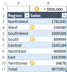
How to highlight sales above and below benchmark using conditional formatting
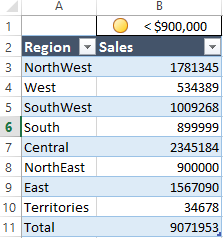
In the summary of regional sales, we are going to highlight the sales above and below $900,000 by adding a yellow light next to the number.
This can be achieved with conditional formatting in Excel. Here is how it is done.
First select the range that you want to format conditionally. In our example above, select B3:B11.
Go to the Home tab and select conditional formatting (for Excel 2007 – 2016). Conditional Formatting is grouped within Style.
In the dropdown list, Choose Manage Rules.
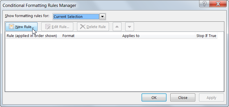
In the pop-up window, select New Rule.
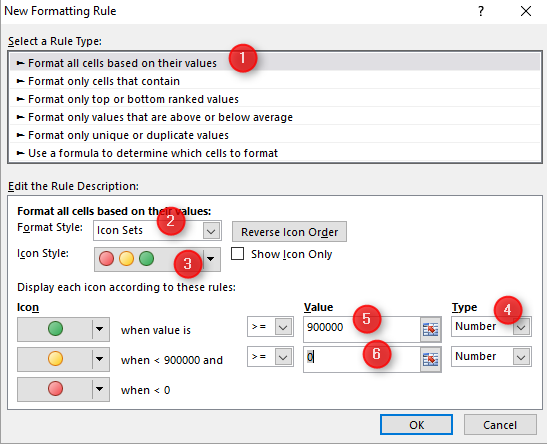
Follow the following steps in the next pop-up window.
1. Select the option “Format all cells based on their values”.
2. Change the Format Style to Icon sets.
3. Select the Icon Style as 3 traffic light (unrimmed) Icon.
4. Select the Number from the Type dropdown list.
5. Type the value for “>=” 900000.
6. Type the value for “>=” 0.
When you have completed the steps, you should get the same setting as shown in the picture below:
Enter the value 900000 into the first conditional rule and set the second conditional rule to 0
Click ok.
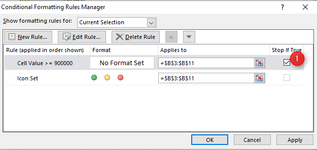
You should see a window as shown below.
Click OK. The yellow & green colours are now displayed in the range from B3:B11.
Now select the same range B3:B11 again to apply another condition format to values above 900000; in this case, greater than or equal to $900,000, and set the format to Automatic. Then, select the Stop If True check box.
Go to the Home tab and select conditional formatting (for Excel 2007 – 2016). Conditional Formatting is grouped within Style.
In the dropdown list, Choose Manage Rules.
In the pop-up window, select New Rule.
Follow the following steps given below in the next pop-up window.
1. Select the option “Format only cells that contain”.
2. Select the option “greater than or equal to” from the dropdown.
3. Type the value “900000”.
4. Click on the format tab.
When you have completed the steps, you will get the same setting as shown in the pictures below:
Click OK. The Yellow colour is now displayed in the column from B3:B11.
How this works:
If rule 1 is true : Excel applies the format, which is set to Automatic (black on white). Nothing changes in those cells visually. Excel will ignore rule 2 because the Stop If True check box is selected.
If rule 1 is false Excel evaluates rule 2:
The yellow icon is applied if the value is >=900,000.
The green icon will not be applied because rule 1 stops evaluating when > 900000.
The red icon will not be applied because there are never any negative values.
New! Comments
Have your say about what you just read! Leave me a comment in the box below.
Share this page:
Enjoy this page? Please pay it forward. Here’s how…
Would you prefer to share this page with others by linking to it?
- Click on the HTML link code below.
- Copy and paste it, adding a note of your own, into your blog, a Web page, forums, a blog comment, your Facebook account, or anywhere that someone would find this page valuable.
<a href=”http://www.advanced-excel.com/”>Advanced Excel – From a Business Perspective</a><a href=”http://www.advanced-excel.com/”>Advanced Excel – From a Business Perspective</a>

Excel Courses for Business Professionals
Copyright © advanced-excel.com 2007 – 2019. All Rights Reserved. Privacy Policy
Microsoft® and Microsoft Excel® are registered trademarks of Microsoft Corporation.
advanced-excel.com is in no way associated with Microsoft


