Vlookup Function
VLOOKUP can look up the related value from another range and show it side by side so that you do not have to toggle between both ranges. The two ranges can be within the same worksheet, different worksheets in the same Excel file or from different Excel files. But I recommended that you do your VLOOKUP within the same Excel file.
The power of VLOOKUP as a worksheet function allows us to match multiple values in one worksheet to the related values in another worksheet. For example, we can match the product code and return the product name located in another worksheet.
The application of VLOOKUP on multiple values is the same as merging the records of two data tables in Data Analytics. Learning VLOOKUP will help you build a strong foundation in data analytics.
Given below is a detailed example of how VLOOKUP works.
The purpose of the vlookup function is to look for a value in a list and returns the results found within the same row of the value (in the 2nd Column, 3rd column , etc) of the list. Vlookup worksheet function will deliver different results, depending on what has been provided in the formula. Therefore it is important that we understand how the vlookup works.
First, let�s start with a simple example #1.
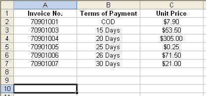
Assuming you have a list given below:

In cell A10, enter the vlookup function given here (without inverted commas):
“=VLOOKUP(70901005,$A$1:$B$7,2)”
You will notice that the cell will return the result “25 days”. It is the value given in Cell B5. Let’s find out what was the instruction given in the vlookup formula that leads to this result.
In the formula, we have indicated in the vlookup formula that we are looking for the value “70901005” vertically (from rangeA1 to A7). When the value is found, it was instructed to return the value in the 2nd column denoted by the number 2 in the formula
“=VLOOKUP(70901005,$A$1:$B$7,2)”.
Note that we have entered the range $A$1:$B$7 into the formula. The range B1 to B7 is included because we need to tell Excel to look for the results within a specific range. If we are to include a larger range into theformula, it will take up more memory as Excel would have to look through more rows for the values.
Now let’s replace the value “70901005” with “70901002” which is not found in the list. In this case, Excel will return the results associated with a value in Column A that is smaller that the lookup value (“70901002”). Since “70901001” is smaller than “70901002”, Excel will accept this value and gives you the results “COD”. Do note that the Invoice No must be arranged in ascending orders (smallest to the largest number) for the vlookup function to work.
If we are to enter the word “false” at the end of the formula like this=VLOOKUP(70901005,$A$1:$B$7,2,FALSE), you will notice that the results turns into “#N/A”. The word “false” has triggered another instruction to Excel. We have indicated that we do not want the vlookup function to return any result if the value (“70901002”) cannot be found. When we omitted this part of the formula, Excel by default assumes that we want to find the closest match to the value. Hence, “COD” wasreturned when we did not enter the word “false” into the formula.
If we are to enter the word “false” at the end of the formula like this
=VLOOKUP(70901005,$A$1:$B$7,2,FALSE)
you will notice that the results turns into “#N/A“. The word “false” has triggered another instruction to Excel. We have indicated that we do not want the vlookup function to return any result if the value (“70901002“) cannot be found. When we omitted this part of the formula, Excel by default assumes that we want to find the closest match to the value. Hence, “COD” was returned when we did not enter the word “false” into the formula.
