Excel’s SUMPRODUCT Formula is BIG Deal!

When I first learned about the SUMPRODUCT formula in Excel, I almost dismissed it as a useless formula used by only few users. How often would anyone need to multiply 2 or more groups of numbers together and add up the results!?

To get to the story, we know that formula is keyed in as:

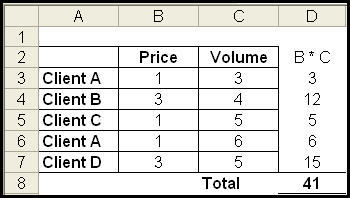
=SUMPRODUCT((B3:B7)*(C3:C7))

This is the same as taking B3 and multiply it by C3, followed by next set

and so on. Then, add up the total derived. The answer is 41. The working is as follows:

Then I found out something really exciting about the formula! Unknown to many Excel users, the formula can actually be tweaked to sum up numbers based on condition(s), for instance, if you have a set of data and you are required to present the (sales) volume of Client A.

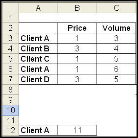
The formula can be entered by equating the ranges to conditions. For example, we can equate range A3 to A7 to A12 (which is Client A) and sum up the values in column B and C that correspond to the rows in Client A. The total is 11, based on the sum of the values in B3, C3, B6 and C6.

Thus, the formula is tweaked as follows to achieve this result:=SUMPRODUCT((A3:A7=A12)*B3:C7)

Question, why do we have to use this if we can also achieve the same result with the SUMIF formula? The reason is, unlike SUMIF, SUMPRODUCT is able to take in more than one condition! This is superb! We can sum up the values of either the pricing column or the volume column if the condition is added into the formula like this:

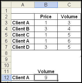
=SUMPRODUCT((A3:A7=A12)*(B2:C2=B11)*(B3:C7))

It will return 9, the total of 3 and 6 in C3 and C6 respectively.

What if you wish to sum up the values of 2 conditions that are in the same column, e.g. Client A and B?

You can use the addition sign to combine the 2 conditions together as shown below:

=SUMPRODUCT(((A3:A7=”Client A”)+(A3:A7=”Client B”))*(B2:C2=B11)*(B3:C7))

Note: SUMPRODUCT will not work if your range of data contains #N/A values or a mixture of text and numbers in the number range. In our example above, that will be B3:C7

The formula wowed me a great deal during the creation of the Excel Calendar. I was using Conditional Formatting to highlight individual cells with the help of VLOOKUP. But when I start to highlight a range of cells using a start date and end date, VLOOKUP fails. That was when I discovered the power of SUMPRODUCT formula which could help me work with multiple ranges and determine if the date falls within the range. It works so perfectly well because I can use one range to determine the open date and another range to determine the close date. Any date that falls outside of the ranges will not be highlighted.

Find out how to calculate the number of working days using the SUMPRODUCT formula.