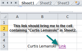
Dynamic Hyperlink

Everyone would agree that creating a hyperlink in Excel is pretty straightforward. All you have to do is to copy the url (web address) from your web browser and paste the link into one of the cells in Excel. Using the INSERT method, you can also create a link that allows you to jump to another worksheet, another cell in the same file. But that is not what we are going to share with you here. We would like to share with you the worksheet function version that can do more than just jumping to another cell in another worksheet or to link to a website. It can help you search for text located in another worksheet.

Basic use of HYPERLINK formula

First let us look at the basic setup of the formula:

There are 2 inputs required for this formula to work.

The first input is the link location and the second is the friendly name, i.e. the displayed name. Supposed you would like to link to a cell C5 in the worksheet Sheet2 from Sheet1. You have to enter the full name of the file followed by the worksheet name and then the cell. Assuming that your file is located in D:everydayExcel MktgMsg_1208, the file name is called search.xls, you will have to enter the formula as

=Hyperlink(“[D:everydayExcel MktgMsg_1208search.xls]Sheet2!C5,”Displayed Name”)

Note that the file directory must be enclosed within the square brackets [xx]

Displayed Name is used to disguise or shorten actual link. It is also commonly known as the anchor text.

Between this worksheet formula and INSERT HYPERLINK formula, I would rather choose the latter which is more straightforward. It’s found in the pop-up menu when we right click within a cell.

So what is use of learning this function?

Combined with other formulas such CELL, ADDRESS, MATCH and Ampersand (“&”), you can turn it as a powerful search function.

Let’s say I have 3 worksheets & I want to put a link in C5 (Sheet1) to find whatever’s in B5 in another worksheet named “Sheet2”.

For the first input which requires the filename and its location on the computer, we can use the CELL formula to automatically return where the Excel file is located.

“Cell(“filename”,[reference]).

The “reference” should be a cell in the worksheet you wish to jump to. In our case, we’ll go to Sheet2 & select A1.

The CELL formula gives the full details for the directory, current Workbook & Worksheet Name as shown.

[D:everydayExcel MktgMsg_1208search.xls]Sheet2

To link it to a cell reference, we need an exclamation mark after the worksheet name & the cell we are looking for. To find the row number “Curtis Lemanski” is at, we can use a MATCH formula:

The “lookup_value” is where “Curtis Lemanski” in Sheet1 is at (i.e. B5). “lookup_array” is a range in Sheet2 where “Curtis Lemanski” is be located. That range is “A1:A15” for our example. And putting “0” in “match type” suggest that we only want to find an exact match.

The ADDRESS formula returns a cell reference when it is given the row number & column number.

Row number has already been obtained by using the MATCH formula while column number is “1”, referring to Column A.

Using the “&”, we combine the filename, worksheet name, “!” and the cell reference to form this:

=HYPERLINK(CELL(“Filename”,Sheet2!$A$1)&”!”&ADDRESS(MATCH(B5,Sheet2!A1:A15,0),1),”Link”)

And we’ll get:”[D:everydayExcel MktgMsg_1208search.xls]Sheet2!$A$6 When we change the name given in B5, the hyperlink will be re-directed to the particular name.